B-Trees vs LSM Trees: Storage Engine Trade-Offs and Compaction Mechanics
Compare B-Tree in-place updates against LSM Tree append-only storage engines: write amplification, Bloom filters, and compaction strategies.
On this page
Every database in production faces the same fundamental challenge: persistent storage on physical disks (whether NVMe SSDs or magnetic media) is orders of magnitude slower than CPU registers and volatile RAM. The way a database organizes data on disk dictates its operational personality: how quickly it can absorb incoming write traffic, how efficiently it can resolve range queries, and how much write amplification it inflicts on physical hardware.
Modern relational and distributed databases converge around two primary storage engine architectures: B-Trees and Log-Structured Merge-Trees (LSM Trees).
B-Trees power the relational backbone of the software industry, including PostgreSQL, MySQL (InnoDB), and SQLite. LSM Trees power the high-throughput write engines of modern distributed stores, including RocksDB, Apache Cassandra, ScyllaDB, and ClickHouse.
This guide provides a deep comparative analysis of B-Trees and LSM Trees: examining page layouts, write paths, read amplification, and the physical engineering trade-offs governing each design.
The Core Structural Difference
The defining distinction between B-Trees and LSM Trees is how they mutate data on physical storage:
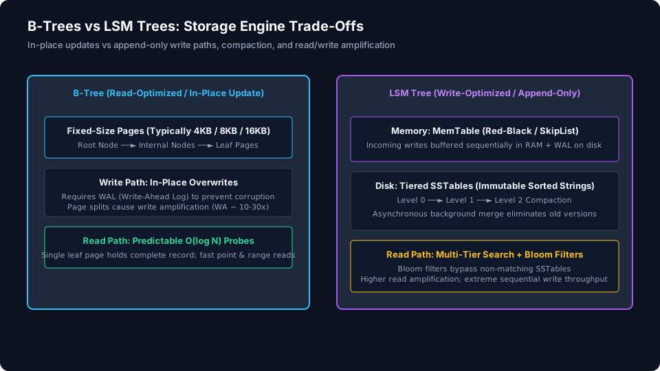
- B-Trees perform in-place updates: Modifying a record updates the specific physical disk page where that record lives.
- LSM Trees perform append-only writes: Modifying a record appends a new immutable mutation to a sequential log; older versions are reconciled later during background compaction.
1. B-Trees: The Read-Optimized Standard
A B-Tree (and its ubiquitous variant, the B+ Tree) organizes data into fixed-size contiguous blocks called pages (typically 4 KB, 8 KB, or 16 KB).
Anatomy of a B+ Tree
- Root and Internal Nodes: Contain routing keys and child page pointers. They fit entirely into memory to guide searches.
- Leaf Nodes: Contain the actual table rows or index record pointers. All leaf pages are linked in a bidirectional doubly linked list, enabling efficient sequential range scans.
                  [ Root Node (Page 1) ]
                  /          |                  [ Page 12 ]    [ Page 13 ]   [ Page 14 ] (Internal Nodes)
          /       \       /      \      /            [ L1 ] <-> [ L2 ] <-> [ L3 ] <-> [ L4 ] <-> [ L5 ] (Leaf Pages)
The In-Place Update Cost
When an application updates a 40-byte column in a 16 KB page, the database must write the entire 16 KB page back to disk.
To prevent corruption if the operating system crashes mid-write (a torn page), the database must first write the modification to a sequential Write-Ahead Log (WAL). Writing 40 bytes therefore incurs:
- Appending to the sequential WAL.
- Writing the dirty 16 KB page back to disk during checkpointing.
This phenomenon is known as Write Amplification (WA):
Write Amplification = Bytes Written to Storage / Bytes Written by UserIn B-Tree systems with random writes, write amplification frequently ranges between 10x and 30x. Furthermore, when a leaf page exceeds its capacity, the storage engine must execute an expensive page split, allocating a new page, shifting half the keys, and updating parent pointers.
2. LSM Trees: The Write-Optimized Machine
LSM Trees eliminate random disk I/O entirely from the write path, converting every insert, update, and delete into contiguous sequential disk writes.
The Write Path: MemTable to SSTables
- MemTable (RAM): Incoming writes are buffered in an in-memory data structure (typically a SkipList or Red-Black Tree) sorted by primary key. Simultaneously, the write appends to a disk WAL for crash recovery.
- SSTable Flush (Disk): When the MemTable reaches a threshold (for example, 64 MB), it is frozen and written to disk as an immutable Sorted String Table (SSTable) at Level 0.
- Deletions via Tombstones: Deletes do not erase data on disk immediately. They append a special marker called a tombstone. The physical data is pruned during background compaction.
Write ──► [ WAL (Disk) ]
      ──► [ MemTable (RAM) ] ──(Flush)──► [ Level 0 SSTable ]
                                                 │
                                                 ▼ (Background Compaction)
                                          [ Level 1 SSTables ]
                                                 │
                                                 ▼
                                          [ Level 2 SSTables ]
3. The Compaction Dilemma
Because SSTables are immutable, an LSM Tree quickly accumulates multiple files containing overlapping key ranges. If key user_102 is updated four times across different flushes, four separate SSTables contain versions of that key.
To prevent disk exhaustion and maintain read performance, the storage engine continuously runs Compaction:
- Merges multiple SSTables into a single sorted SSTable (like mergesort).
- Discards overwritten values and purges deleted rows matching tombstones.
Compaction Strategies
- Size-Tiered Compaction: Merges SSTables of roughly equal size together. Prioritizes high write throughput, but incurs high temporary disk space overhead (space amplification up to 50%).
- Leveled Compaction (RocksDB default): Divides disk into hierarchical levels (L1, L2, L3), where each level is 10x larger than the previous. Guarantees that key ranges within each level never overlap, optimizing read latency at the expense of higher background write amplification.
4. The Read Path: Why LSM Trees Need Bloom Filters
In a B-Tree, finding a key requires traversing log_B(N) pages. Because internal nodes are cached in RAM, resolving a point query usually takes a single disk read.
In an LSM Tree, finding a key naively requires searching the active MemTable, followed by probing every SSTable across all levels until the key is found. If a key does not exist, the engine would have to read every single SSTable on disk!
To solve this read amplification, LSM Trees employ Bloom Filters:
- A probabilistic bit array is maintained in memory for every SSTable on disk.
- If the Bloom filter returns
false, the engine knows with mathematical certainty that the key does not exist in that SSTable, skipping the disk probe entirely.
Architectural Comparison Matrix
| Dimension | B-Tree (e.g., PostgreSQL, InnoDB) | LSM Tree (e.g., RocksDB, Cassandra) |
|---|---|---|
| Primary Workload Fit | Read-heavy, complex range scans, low latency. | Write-heavy, time-series, event streams, append-only logs. |
| Write Strategy | In-place random page updates + WAL. | Sequential append to MemTable + immutable SSTables. |
| Write Amplification | High (10x to 30x due to full page rewrites). | Low to Moderate (low initially; elevated during compaction). |
| Read Latency (P99) | Predictable and consistent (single page probe). | Variable (requires probing multiple SSTables if cache misses). |
| Disk Space Overhead | Low (fragmentation occurs, but minimal duplication). | Higher (transient space spikes during compaction). |
| Hardware Wear (SSDs) | High write wear on flash memory blocks. | Low write wear; sequential writes maximize SSD longevity. |
Practical Selection Guide
- Pick B-Trees when: Your workload is read-dominated ($> 80%$ reads), transactions demand strict ACID multi-row guarantees, and predictable sub-millisecond point-read latencies are non-negotiable.
- Pick LSM Trees when: Your application ingests massive streams of telemetry, time-series metrics, financial tick data, or event logs where write throughput exceeds disk IOPS limits.
Keep reading
Relational Database Design Guide: Keys, Relationships, Normalization, and Joins
A comprehensive guide to relational schema design, primary and surrogate keys, normal forms (1NF to BCNF), and indexing join performance trade-offs.
How CockroachDB Built Distributed Vector Indexing at Scale
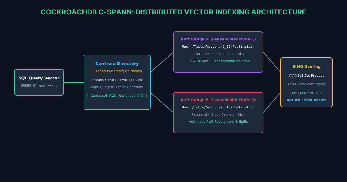
Inside C-SPANN, CockroachDB's distributed vector index stored as ordinary table rows to achieve fresh, transactional vector search without memory blowup.

How Instacart Built a Search Engine for Billions of Items on PostgreSQL
How Instacart migrated product search from fragmented Elasticsearch clusters onto a unified PostgreSQL and pgvector stack to eliminate sync lag.
/* Comments */
Comments are offline right now — we reconnect automatically, nothing is lost.