Why Google Maps Computes Shortcuts Offline

A phone call comes in: “Get me from San Francisco to New York.” The algorithm has 65 million road intersections in North America to consider. A naive Dijkstra expansion from the origin will fan out into every neighbourhood, every alley, every cul-de-sac before any path reaches the destination 2,500 miles away. Running this in 10 milliseconds isn’t possible. So Google Maps does not run Dijkstra at all—instead it runs something at query time that only looks like Dijkstra, because the hard work was done offline.

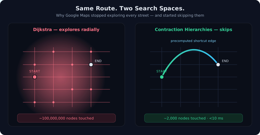The breakthrough: a precomputed shortcut edge skips 100 million node expansions.

The Naive Way: Dijkstra Explores Everything

Dijkstra’s algorithm is correct and elegant: maintain a priority queue of distances from the origin. Pop the closest unexplored node, relax its outgoing edges, repeat until the destination is reached. On a road graph with 65 million nodes representing North America, this means:

1. Pop the origin (San Francisco).
2. Relax all edges to nearby intersections: add them to the queue.
3. For the next ~100 million expansions, pop the globally-closest-so-far node and expand its neighbours.
4. Eventually reach New York and backtrack the shortest path.

Every street gets considered—neighbourhood avenues, parking-lot entrances, dead ends, rural highways in Nebraska—because the algorithm has no information about which edges lead toward the destination 2,500 miles away. It only learns that information by exploring. On a modern CPU, 100 million node operations take perhaps 2–3 seconds. But a user calling “Get me directions” expects the response in under 100 milliseconds.

Why not just parallelize Dijkstra or use a faster heap? Because the cost isn’t the heap operations—it’s the node visits themselves. Each node you pop from the queue forces you to examine its outgoing edges, update distances, and push new nodes. On a dense graph, this is unavoidable overhead. A city intersection might have 5 outgoing roads; a highway junction might have 8. Multiply by 65 million nodes and you’re stuck.

The real problem is fundamental: Dijkstra must touch nodes in order of distance, and distance from San Francisco to every street in America is expensive to compute. The only solution is to not visit most nodes.

The Breakthrough: Contraction Hierarchies

Contraction Hierarchies solves this by asking: which nodes must be visited during a shortest-path query? The answer is highway intersections—Interstate on-ramps, major junctions. A shortest path from San Francisco to New York will use Highway 80, then Interstate 80, then Highway 395, then local streets at the destination—it will not explore local streets in Reno or Nebraska. But a naive algorithm doesn’t know this; it has to learn by exploring.

The key insight: offload the learning to precomputation. Before any query arrives, compute an ordering of nodes and precompute the shortcut edges they imply. A shortcut edge encodes “the shortest path from A to C that does not touch B”—the algorithm never needs to touch B during a query because the answer is already in the graph.

The mechanism is node contraction. You iteratively remove nodes from the graph in a chosen order. When you remove a node B with incoming edges from {A, C, D, …} and outgoing edges to {E, F, G, …}, you create shortcut edges directly from each incoming neighbour to each outgoing one, preserving the shortest-path distance. If the shortest path from A to E was A→B→E with weight 27, then a shortcut A→E gets weight 27. After contraction, you can ignore B entirely—any query routing through that region will use the shortcut instead.

The strategy is: contract the nodes that matter least first. “Matters least” means low-degree nodes—intersections with few connections. In a road network:

• A cul-de-sac (degree 1) contributes zero shortcut edges because its sole connection is to the rest of the graph.
• A neighbourhood intersection (degree 3–4) contributes ~10–20 shortcuts when removed.
• A highway junction (degree 8) contributes ~32 shortcuts when removed.

By contracting low-degree nodes first, you build up shortcuts gradually without explosion. After contracting all the neighbourhood streets, a single city block is reduced to a handful of shortcuts connecting to the regional network. By the time you reach highway junctions, all the local topology is already encoded as shortcuts; contracting the highway node adds only edges to other highway-level nodes, which is much smaller.

How It Works: Step by Step

Precomputation happens once, offline:

1. Rank all nodes by a heuristic that approximates importance. One approach: assign a random rank (surprisingly, this works well). Another: use degree + centrality + proximity to highways. The exact heuristic matters for compression ratio but not correctness.

2. Contract nodes in rank order. For each node i in rank 1 to N:

   • Find all pairs (u, v) such that a path u→i→v exists (u is an incoming neighbour of i, v is an outgoing neighbour).
   • For each pair, compute dist(u, v) = dist(u, i) + dist(i, v).
   • If no existing edge u→v has weight <= this distance, create a new shortcut edge u→v with weight = dist(u, i) + dist(i, v).
   • Remove node i from the graph.

3. Assign hierarchy levels. After contraction, node i has level = max(level of its incoming neighbours at contraction time) + 1. This encodes the contraction order into the graph itself.

Query time uses a modified bidirectional Dijkstra:

• Expand from both source and destination simultaneously.
• When expanding upward from the source, only relax edges to nodes with strictly higher hierarchy level.
• When expanding downward from the destination, only relax edges to nodes with strictly higher hierarchy level.
• Stop when the two search frontiers meet.

This achieves the skip: a query from a cul-de-sac (level 1) to a neighbouring street (level 2) expands only a local subgraph because there are no edges to higher levels. A coast-to-coast query expands upward through hierarchies (cul-de-sacs → neighbourhoods → city regions → highways) until both searches meet at highway-level nodes, where precomputed shortcuts encode the long-distance path. Most of the graph is skipped.

The number of nodes touched scales with the height of the hierarchy, not the graph size. For a continent-scale road network, hierarchy depth is roughly log(N) to constant factors (because most shortcuts are created early when contracting low-degree nodes). This is why queries are consistently fast regardless of whether the origin and destination are 10 miles or 2,500 miles apart.

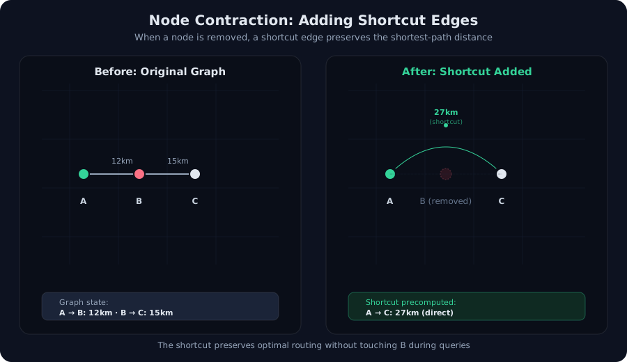When node B is contracted, a shortcut edge A→C preserves the distance without exploring B during queries.

The Trade-off: Memory for Speed

Precomputing shortcuts is expensive in both space and time. A road graph with 65 million nodes and ~70 million edges grows to roughly 1 billion shortcut edges—about 14× the original size. Each edge is a triple (from-node, to-node, weight), so this is ~36 GB in a naive representation. Practical systems compress it using:

• 32-bit node indices instead of 64-bit pointers.
• Varint-encoded weights (traffic delays compress well because adjacent roads have similar times).
• Adjacency-list layouts instead of edge lists (store outgoing edges in order by node ID).

Real-world deployments fit this into 1–4 GB in RAM on a single server. On-disk, with additional compression, it’s under 500 MB.

Query latency: sub-millisecond for point-to-point routing. You touch ~2,000 nodes instead of 100 million. This is the direct trade-off: storage and precomputation time for query speed.

Precomputation itself takes 10–30 minutes on modern hardware for a continent-scale network. The fastest implementations use GPU-accelerated sorting and parallel edge insertion. This is done once per week or per day; the result is pushed to query servers.

Contraction Hierarchies also has a failure mode: dynamic graphs are expensive. If a road closes or traffic conditions change significantly, the precomputed shortcuts are still mathematically correct (they encode true shortest paths under the original weights), but they don’t account for the new state. Real-world systems handle this by:

• Using weighted graphs where each edge has a current-weight multiplier (traffic factor), and shortcuts multiply the entire path weight. The shortcut distance is still optimal; it’s just time-dependent.
• Reprecomputing shortcuts on a schedule (daily, or on major infrastructure changes) rather than in real-time.
• Blending Contraction Hierarchies with customizable route planning (CRP) for fast replanning after closures without full recomputation.

When Not to Use It

Contraction Hierarchies shines for static, dense road graphs where query latency is critical and precomputation cost is amortized over millions of queries. It is overkill or infeasible if:

• Small graphs: a building, campus, or city network. Dijkstra is fast enough (< 50 ms) and doesn’t need precomputation overhead.
• Highly dynamic graphs: task scheduling, peer-to-peer networks, graphs that change by the second. Precomputation breaks because recomputing hourly or daily is too expensive. Opt for plain Dijkstra or A* with a good heuristic.
• All-pairs queries: if you need shortest paths between every pair of nodes, precomputation buys you nothing—you still need to answer N² queries. Standard solutions include Floyd-Warshall (for small N) or storing the matrix (for very small graphs).
• Memory-constrained environments: the 14× overhead is real. On a phone or embedded system, this is infeasible.
• Frequent graph updates with query mixing: if you need to handle edge-weight changes (like real-time traffic) and structural changes (closures), the precomputed hierarchy becomes stale. Hybrid approaches exist (e.g., customizable route planning) but are more complex.

Alternatives for different constraints:

• Faster-than-Dijkstra on small graphs: A* with Euclidean distance heuristic (or landmark-based lower bounds).
• Fast queries on dynamic graphs: Hub Labels (precomputes hub sets per node; answers queries in microseconds but recomputation is still expensive). Customizable Route Planning (CRP) precomputes a partial hierarchy that can be customized per query for different weights without full recomputation.
• Massive-scale graphs: the hierarchy approach scales, but for billion-node graphs (the entire internet), even hierarchical compression is pushed to distributed systems (Google Spanner, etc.).

The Lesson

Routing 100 million nodes in 10 milliseconds looks impossible until you realize: you don’t have to explore them. By precomputing an ordering and using it to structure the graph into a hierarchy, you reduce the search-space complexity from O(N + M log N) to roughly O(log N) node expansions. The problem changes from “visit 100 million nodes” to “visit 2,000 nodes and read precomputed edges.”

The key insight that makes this work: the precomputation is correct—it encodes true shortest-path distances, not approximations. Shortcuts are not heuristic guesses or lossy compression; they are mathematical truths derived from the original graph. A query can skip entire regions because the shortcuts prove that no optimal path runs through them at the neighbourhood level—optimal paths must use the highway hierarchy.

This is why Google Maps, OpenStreetMap’s routing engine, and every production map service uses some variant of Contraction Hierarchies or its descendants (Hub Labels, Customizable Route Planning, Transit Node Routing). The basic idea is simple enough to fit on a whiteboard: rank nodes, contract low-rank ones first, encode the hierarchy in the graph. The impact is enormous: 100 million → 2,000 nodes, 3 seconds → 10 milliseconds. And it is invisible to the user—they ask for directions and get an answer instantly, without any sense of the computation happening offline or the hierarchy being consulted.