LSM-Trees vs B-Trees: Why Cassandra Chose Sequential Writes

You have 10 million write requests per second. A B-tree database would seek its disk-head 10 million times. A 7,200 RPM disk makes maybe 100 random seeks per second before the controller queue backs up and requests time out. Cassandra, RocksDB, and Bigtable solved this not by buying faster disks, but by changing how they write to them.

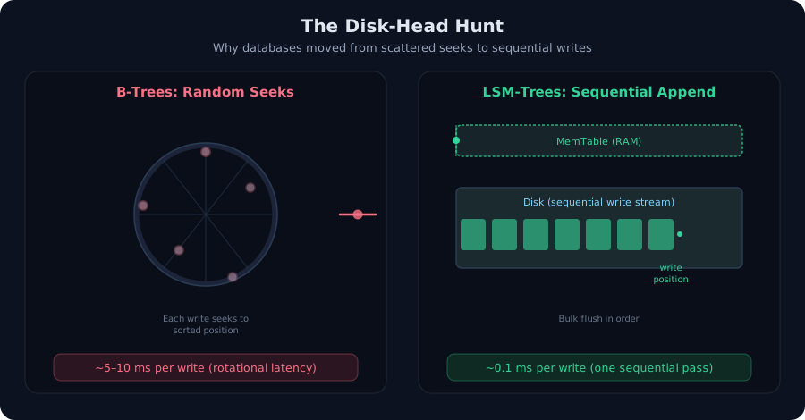Left: B-trees perform a disk seek for each write, touching the platter sequentially but at random positions. Right: LSM-trees buffer writes in memory and flush them in one sequential pass, converting random I/O into bulk sequential writes that sustain 100x higher throughput.

Why B-Trees Fail Under Write Load

A B-tree is a sorted data structure: pointers branch left for smaller keys, right for larger. To insert a new key, the tree finds its sorted position and writes it to disk. That sounds simple—but “write to disk” means:

1. The disk controller seeks the arm to the correct cylinder
2. The platter rotates to the correct sector
3. The write happens

On a mechanical drive, step 1 alone takes 5–10 milliseconds. Modern SSDs are faster (0.1–1 ms), but solid-state storage still has fundamental write limits: flash cells degrade with use, and amplification from the flash translation layer adds overhead.

The result? A B-tree implementation struggles to exceed 1,000–10,000 writes per second, regardless of CPU or network speed. The disk becomes the bottleneck—not because it’s slow, but because you’re using it wrong.

The LSM Breakthrough: Write First, Sort Later

Log-Structured Merge-trees invert the write strategy: instead of finding the sorted position immediately, buffer writes in memory, then flush them to disk in sorted bulk operations.

The pipeline:

1. MemTable (in RAM): Incoming writes go to a sorted data structure in memory (often a skip list or B-tree). The MemTable is tiny, just 2–4 MB per server.
2. SSTable flush: When the MemTable fills, it’s written to an immutable file on disk called an SSTable (Sorted String Table). This is a sequential write—one pass, no seeking.
3. Compaction: As SSTables accumulate, overlapping ranges are merged into fewer, larger SSTables on higher levels. Duplicates are removed, deleted keys are discarded.

This simple reordering—sort in memory first, write sequentially, then organize on disk—converts random I/O into sequential I/O. A single sequential pass writes gigabytes per second; the same disk doing random seeks writes megabytes per second.

Result: LSM-trees sustain millions of writes per second, limited by CPU and network bandwidth, not disk seeks.

The Mechanism: MemTable to Compaction Levels

The LSM write pipeline: writes accumulate in a MemTable; when full, it flushes to Level 0 as an immutable SSTable. Overlapping files are compacted into a higher level, merging and removing duplicates. This trades write amplification against read amplification.

Write Path

Every write hits the MemTable first—a fast in-memory structure. Optionally, it’s also logged to disk (a write-ahead log or journal) for crash recovery. The MemTable holds maybe 2 MB before flushing; at a typical write size of 1 KB, that’s 2,000 writes before a flush.

When the MemTable fills:

1. A new MemTable opens for incoming writes
2. The old MemTable is flushed to disk as an immutable SSTable
3. This flush is sequential—one sorted stream to disk

A flush takes milliseconds, and multiple flushes can queue without blocking new writes.

Read Path (The Problem)

This is where LSM-trees pay the bill. A read must search multiple SSTables:

• Level 0 has newly flushed SSTables (often 2–10 files, overlapping key ranges)
• Level 1 has older, larger SSTables (10–100 files, mostly non-overlapping)
• Level 2 has even older data (100+ files)

In the worst case, the key might not exist—and the read must check every level before returning “not found”. This is read amplification: more files to search, more I/O.

Without mitigation, a read might need to:

1. Check the MemTable (memory, fast)
2. Check 10 Level 0 files from disk (overlapping, might have the key)
3. Check 100 Level 1 files from disk (mostly don’t have it, but maybe)
4. Check 1,000 Level 2 files from disk (probably not, but must verify absence)

If each file is 2 MB and you have to read them sequentially, that’s 4 GB of disk reads to prove the key doesn’t exist. LSM-trees would be unusable for lookups if this happened regularly. Fortunately, it doesn’t—because of compaction and Bloom filters.

Compaction: The Hidden Cost

Compaction solves the read problem by merging overlapping SSTables into fewer, larger SSTables at higher levels. Instead of 1,000 small files scattered across levels, you end up with a tiered structure:

• Level 0: 2–4 SSTables (recently flushed)
• Level 1: 10 SSTables (merged, non-overlapping key ranges)
• Level 2: 100 SSTables (further merged)

The tiering is exponential: each level is roughly 10x larger than the level below.

The write amplification trade-off: Compaction itself writes data multiple times. A key might be written:

1. As an insert to the MemTable (no I/O, just RAM)
2. As part of a flush to Level 0 (one write to disk)
3. As part of a compaction from Level 0 to Level 1 (read + rewrite)
4. As part of a compaction from Level 1 to Level 2 (read + rewrite)

This multiplies the I/O work. A single 1 KB write from the user becomes 3–5 KB written to disk. Cassandra and RocksDB both experience write amplification factors of 3x to 10x depending on the data model and compaction strategy.

Is it worth it? Yes. You’re trading CPU (compaction runs in the background, on a different thread) and disk space (temporary duplicates during merging) to achieve 100x higher write throughput. A database that writes 100,000 ops/sec can afford to write 300,000 KB/sec to disk; the disk bandwidth is available, and the trade is favorable.

When NOT to Use LSM-Trees

LSM-trees excel at write-heavy, high-throughput workloads. Cassandra and RocksDB are LSM-based because they target 100,000+ writes/sec.

But LSM-trees have weaknesses:

• Read latency is unpredictable: A read might hit memory (microseconds) or require merging 10 SSTables (milliseconds).
• Space overhead: Compaction produces temporary copies of data; you need ~2x the data size in free disk space.
• Deletes are expensive: Deletions don’t erase data immediately—they mark it as deleted (tombstones), and the data lingers until compaction.

Use B-trees when:

• Reads and writes are balanced
• You need consistent, predictable latency
• The workload is transactional (OLTP): many small updates with ACID guarantees
• Examples: PostgreSQL, MySQL, MongoDB (with the default engine)

Use LSM-trees when:

• Writes vastly outnumber reads (write-heavy)
• Throughput matters more than latency consistency
• The workload is analytical or logging: append-heavy with occasional range scans
• Examples: Cassandra, RocksDB, HBase, Bigtable

A modern hybrid approach: RocksDB and LevelDB (LSM-based) are embedded in Chrome, Linux, many mobile apps, and analytical databases like Clickhouse. Bigtable and Cassandra are cloud-native LSM systems designed for write-heavy services. PostgreSQL and MySQL use B-tree variants (B+trees) for OLTP workloads where reads are common.

The disk-head doesn’t care which algorithm you choose—it cares about whether you seek randomly or sequentially. LSM-trees won the write-heavy game by optimizing for sequential I/O.