Why Uber Tiles the Planet in Hexagons

On a sphere, a grid must break somewhere. Mercator projections and lat/long rectangles distort near the poles—Greenland balloons to continent size, Alaska stretches, and grid cells compress into useless slivers. Uber processes billions of rider and driver locations every day across every latitude, and storing them as floating-point {lat, long} coordinates means every “find nearby” query runs expensive trigonometric distance math. In 2016, they released H3: a spatial index that tiles the entire planet in nested hexagons. Six neighbors, equidistant, at every zoom level. A rider’s location becomes a 15-character string cell ID. Finding nearby drivers becomes a hash table lookup. No floating-point math. No sorting. No distance calculations. Just six O(1) probes.

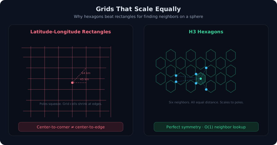The naive way (rectangles distort; neighbors are not equidistant) versus the breakthrough (hexagons scale to the poles and maintain perfect symmetry at all resolutions).

The naive way: rectangles and trigonometry

A straightforward approach: store each driver and rider as a {latitude, longitude} pair. To find nearby drivers, compute the Haversine distance to every indexed driver and sort by distance. This works locally. It breaks at scale.

First, there’s distortion. A degree of longitude near the equator spans roughly 111 kilometers. At the North Pole, a degree of longitude spans 0 kilometers—all longitudes converge to a point. Any rectangular grid built on lat/long coordinates shrinks as you move poleward. A uniform grid cell in Manhattan is a ribbon-thin sliver over Oslo.

Second, there’s inconsistency. In a square grid, the center-to-corner distance is longer than the center-to-edge distance by a factor of √2. This means “find all cells within distance R” can require anywhere from 5 cells (if you search orthogonally) to 12+ cells (if you search diagonally), and the answer changes depending on direction. For a spatial index, this makes it hard to define what “nearby” means and harder still to build efficient algorithms around it.

Third, there’s computation. Every query that checks “is this driver within 500 meters of the rider” requires computing a real distance using the Haversine formula (which involves trigonometric functions and square roots). At Uber’s scale—billions of location updates per day, millions of concurrent queries—that math adds up. Each query touching thousands of drivers multiplies the cost.

The breakthrough: hexagons on a sphere

Hexagons solve all three problems at once.

A hexagon has six neighbors, and—crucially—all six neighbors are equidistant from the center. This isn’t true by accident; it falls out of the geometry. If you tile a plane with regular hexagons, each hexagon’s center-to-neighbor distance is the same in all six directions. And if you project that tiling onto a sphere (the surface of the Earth), the property holds across all latitudes and longitudes. Near the poles, the hexagon sizes shrink just like squares would, but the neighbor relationship remains symmetric.

Uber’s H3 system divides the Earth into 16 hierarchical precision levels (L0 to L15). At the coarsest level (L0), there are exactly 122 hexagons covering the entire planet. At level 9—roughly 174-meter cells—there are 5.2 trillion hexagons. Each cell’s ID is a string like 89283470badcfff, and the hierarchy is baked into the string: strip the last character and you get the cell’s parent at level 14; strip one more and you get the parent at level 13, and so on.

A rider’s GPS coordinates {37.7749, -122.4194} (San Francisco) are hashed using a proprietary algorithm into an H3 cell ID at a chosen precision level (often L9 for driver matching). The hash is deterministic: the same coordinates always map to the same cell, and nearby coordinates map to the same cell or one of its six neighbors.

Mechanism: hierarchical string IDs for O(1) lookups

Here’s how a matching query works in practice:

1. Hash the rider’s location. Take their GPS coordinates and run H3’s hashing function to get their cell ID at L9: a string like 89283470badcfff. This is O(1).

2. Find the region using the parent cell. Extract the first 13 characters: 89283470badcf. This is the L8 parent cell. All drivers within a wider region (city block, neighborhood) have the same L8 parent. Index a hash table by L8 parent; you now know which region to query and whether surge pricing applies. O(1) lookup.

3. Query the six neighbors. Generate the six L8 neighbor cell IDs from the parent. The H3 library provides this in O(1) time—it’s a lookup into a precomputed table of neighbor offsets. For each neighbor, probe a hash table of “drivers in this cell” and collect results. Six probes, each O(1).

4. No distance sorting needed. Because all six neighbors are equidistant, the driver closest to the rider is guaranteed to be in one of these seven cells (the rider’s cell + six neighbors). You don’t need to compute real distances or sort by Haversine; you’ve already found the candidates with the lowest latency.

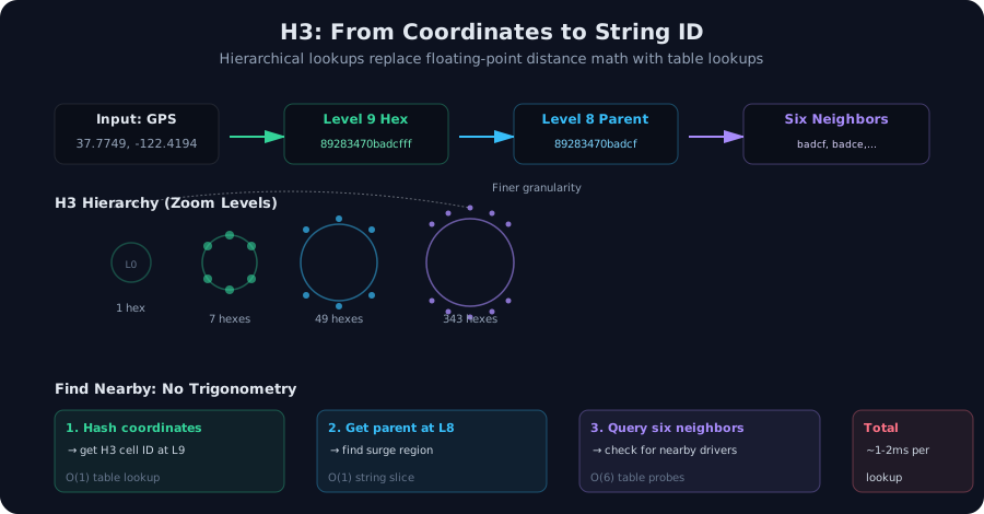H3 converts floating-point coordinates into a hierarchical string ID in one hash, making all subsequent operations table lookups instead of geometric calculations.

The result: finding candidates for a ride match takes microseconds. Surge-pricing calculations—“which cells have demand above the threshold?”—are region table lookups. Delivery zones, geofences, heat maps: all implemented as cell-ID set operations instead of spatial joins.

Trade-offs and limits

Quantization is the price. A driver at the edge of cell A and a rider at the edge of cell B might be 10 meters apart; a driver deep in cell C and a rider deep in cell D might be 1 kilometer apart. Both pairs are in different cells, so both are treated as equidistant neighbors. The acceptable error depends on the cell size: H3 levels 8–10 (174 meters to 5 kilometers) work for most ride-hailing; higher precision levels are used for delivery and logistics.

This works because the problem is probabilistic. You don’t need the single closest driver—you need a good candidate in under 100 milliseconds so the rider can be matched and notified. Quantization error of ±200 meters is invisible at the user’s scale and buys you orders of magnitude in query latency. In a continuous-distance approach, you’re sorting thousands of candidates by exact distance and spending milliseconds doing math. With H3, you’re probing seven hash buckets and picking the first non-empty one.

Parent-cell lookups can be wrong if the region contains a border. A rider and driver on opposite sides of a surge-zone boundary might have different L8 parents. H3 handles this by querying not just the seven cells but also checking the parents’ neighbors when needed. This adds a few extra table probes but keeps the approach fast—still microseconds per query, not milliseconds.

Finally, precomputation and maintenance are required. Drivers must be indexed and re-indexed as they move. Uber maintains real-time indexes of driver positions grouped by cell ID; on each location update, a driver is removed from one cell’s bucket and inserted into another. For a system processing millions of updates per second, this is built into the stream-processing pipeline, not an afterthought. It’s not free—Redis or an in-memory hash table needs capacity—but the cost is far lower than recomputing spatial indexes on every update.

H3 has become the de facto standard for spatial indexing at ride-hailing and delivery companies. Its core insight—that you can trade floating-point precision for discrete cell lookups and gain orders of magnitude in latency—has influenced indexing approaches far beyond Uber. For any system matching distributed agents to requests across a geographic region, hexagonal hierarchical indexing is worth the implementation cost.